Conv-Transformer Representation Learning for 32-Band Hyperspectral Pixel Classification 北京航空航天大学机器学习（宇航学院）课程小组大作业

北京航空航天大学机器学习（宇航学院）课程小组大作业。

有些文章只以英文提供。Some articles are only available in English, and this is one of them.一部の記事は英語でしか利用できません。これもその一つです。

This post records our group project for fine-grained land-cover classification from hyperspectral pixel spectra. The code is available at KohakuKirisame/group-task4-Hyperspectral. The short version is simple: each pixel gives us a 32-dimensional spectral vector, and we ask a neural model to infer the land-cover class from that spectrum alone. The longer version, naturally, involves a convolutional stem, a Transformer encoder, an autoencoding auxiliary task, class imbalance, memmap files, and the ancient machine-learning ritual of watching TensorBoard curves while pretending to be calm.

Task: 32 Bands, One Pixel, One Label

The dataset consists of hyperspectral observations covering approximately 400-1000 nm. For every pixel, the input is a reflectance vector

$$x = [b_1, b_2, \ldots, b_{32}] \in \mathbb{R}^{32},$$

and the target is a land-cover label. The evaluation metric is pixel-level Overall Accuracy (OA). In other words, the model is not given explicit spatial context such as neighboring patches; it must classify a pixel from its spectral signature only.

This setting is both attractive and slightly cruel. It is attractive because a pixel spectrum is compact and easy to batch. It is cruel because many land-cover categories are spectrally similar, while samples from the same category may vary due to illumination, material mixture, atmospheric effects, or plain old measurement noise. A successful model therefore needs to capture both local spectral shapes, such as slopes and absorption-like patterns among adjacent bands, and long-range dependencies across the full spectrum.

The repository README notes a practical detail worth checking before training: the code uses num_classes=5 in several places, while the task description mentions labels in the range 0-5. For a fresh run, the correct number of classes should be verified from the actual label file. The most dangerous bugs are often not dramatic; sometimes they just sit quietly inside a constructor argument.

Main Idea: Local Spectral Shape Meets Global Attention

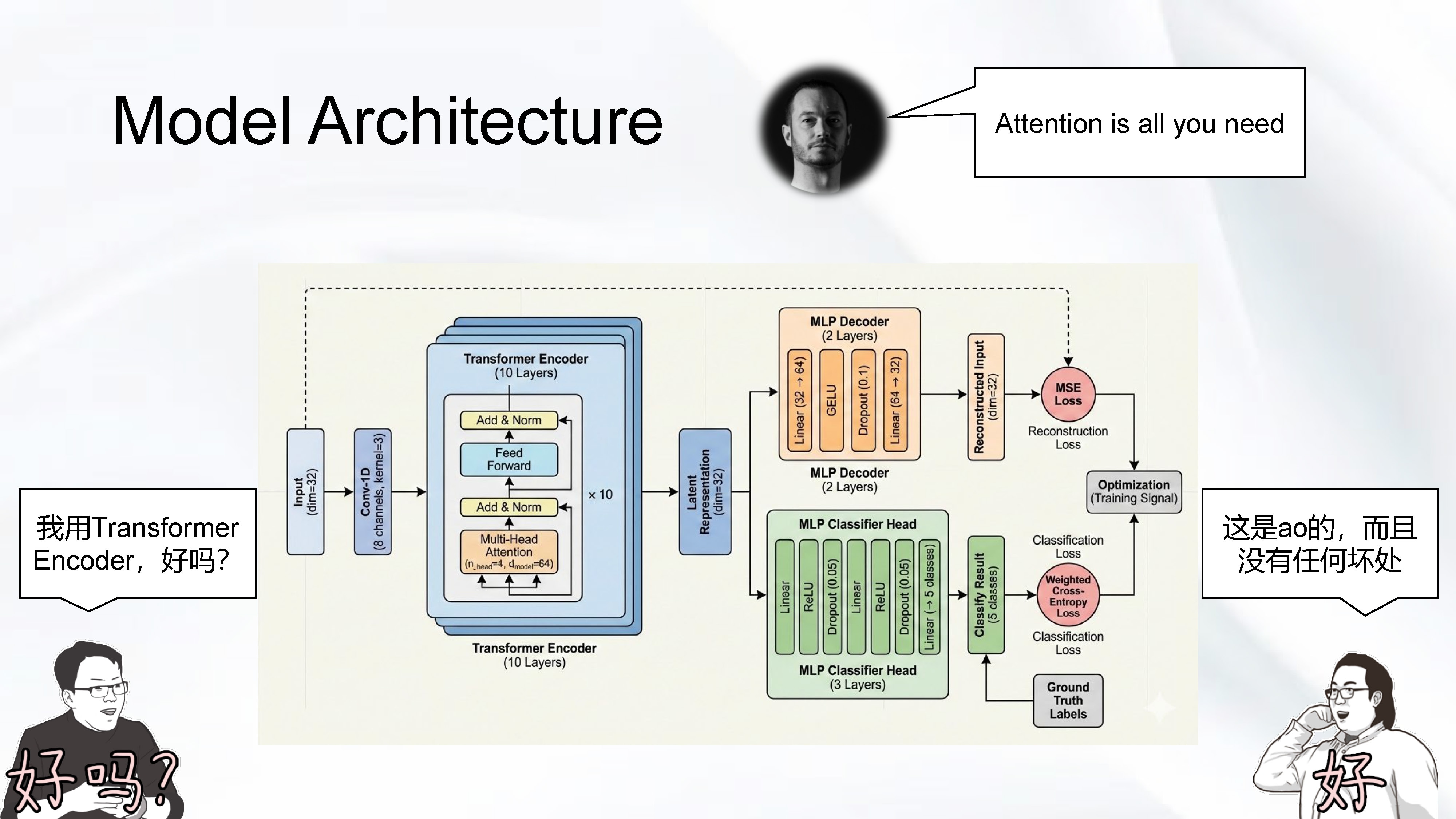
Our model follows a multi-task representation-learning design:

$$\text{input spectrum} \rightarrow \text{shared encoder} \rightarrow \begin{cases} \text{reconstruction head} \\ \text{classification head} \end{cases}$$

The shared encoder is a Conv-Transformer encoder. It first uses a 1D convolutional stem along the spectral axis, then applies a Transformer encoder to model cross-band interactions. The resulting latent vector is used for two objectives:

1. reconstruct the original 32-band spectrum with an MLP decoder;
2. predict the land-cover class with an MLP classifier.

This is the central hypothesis of the project: a supervised classifier benefits from an auxiliary self-supervised reconstruction signal, because the latent space is encouraged to preserve meaningful spectral information rather than only memorizing label shortcuts. In less formal language, the model is asked not only to answer the exam question, but also to prove it has actually read the spectrum.

Architecture

The implementation in custom_model.py defines three main modules: ConvTransformerAE, CustomClassifier, and AEClassifier.

The autoencoder starts with a 1D convolution:

nn.Conv1d(
    in_channels=1,
    out_channels=conv_channels,
    kernel_size=3,
    stride=1,
    padding=1,
)

This layer treats the 32 bands as a short sequence and aggregates local spectral neighborhoods. The convolutional output is transposed into sequence format, embedded into a Transformer dimension, and combined with a learnable positional embedding. The Transformer encoder then learns global relationships among spectral bands:

nn.TransformerEncoderLayer(
    d_model=d_model,
    nhead=n_head,
    dim_feedforward=d_model,
    dropout=dropout,
    batch_first=True,
)

After the Transformer stack, mean pooling over the spectral sequence produces a compact representation, which is projected into the latent space. In the AE pretraining notebook, one configuration uses latent_dim=16, conv_channels=4, d_model=32, and num_layers=3. In classifier training and evaluation, a larger configuration is used: latent_dim=32, conv_channels=8, d_model=64, and num_layers=10.

The decoder is intentionally simple: an MLP maps the latent vector back to the 32 original bands. The classifier is also an MLP with GELU activations and dropout, producing class logits from the latent vector.

The combined classifier wrapper performs:

$$z = f_\theta(x), \quad \hat{x} = g_\phi(z), \quad \hat{y} = h_\psi(z).$$

The training loss is a weighted combination of classification and reconstruction:

$$\mathcal{L} = \mathcal{L}_{CE}(\hat{y}, y) + \alpha \mathcal{L}_{MSE}(\hat{x}, x).$$

The written report uses alpha=0.5 as the experimental setting. The repository implementation in custom_trainer.py currently uses 0.2 * reconstruction_loss during classifier training. Both express the same design principle: cross-entropy defines the supervised decision boundary, while reconstruction regularizes the representation.

Data Pipeline

The raw CSV files are large enough that loading everything naively is not ideal. The project therefore converts CSV files into NumPy .npy memmap arrays. This is a useful engineering choice: it allows the training pipeline to read large feature matrices without keeping the entire dataset in RAM.

The expected training format is:

id, band_1, band_2, ..., band_32, label

and the expected test format is:

id, band_1, band_2, ..., band_32

The preprocessing notebook data_utils.ipynb demonstrates:

1. counting rows in CSV files;
2. streaming rows into features.npy, labels.npy, and test feature arrays;
3. estimating feature-wise mean and standard deviation;
4. writing normalized arrays such as features_norm.npy and test_features_norm.npy;
5. reserving the first 10,000 samples as a validation split.

One important note from the README is that test features should be normalized with training-set statistics. Estimating mean and standard deviation from the test set may look harmless, but it leaks distribution information into evaluation. Leakage is like seasoning: a tiny amount changes the whole dish, and reviewers tend not to enjoy it.

The dataset class is deliberately lightweight. CustomDataset opens feature and label arrays with np.load(..., mmap_mode="r"), then returns PyTorch tensors. An optional offset is used to skip validation samples when constructing the training loader. For inference, EvalDataset returns (sample_id, x), although the current implementation uses the array index as id; if real test IDs are not continuous from zero, they should be saved and restored explicitly.

Training Procedure

The project is organized into a notebook-driven workflow.

Step 1: Autoencoder Pretraining

The autoencoder is trained on normalized spectra using MSE reconstruction loss. The notebook trainer.ipynb uses:

• batch_size=4096;
• AdamW with lr=1e-4;
• weight decay around 1e-4 in the code;
• StepLR scheduling, stepped per optimization step;
• 5 training epochs in the recorded run.

The autoencoder checkpoint is saved as:

resources/models/model_{epoch}.pth

This stage learns a spectral representation before forcing the model to care about class labels. In representation-learning terms, the reconstruction task provides a self-supervised prior: the latent vector must preserve enough information to rebuild the spectrum.

Step 2: Classifier Training

The classifier stage wraps the pretrained autoencoder with an MLP classification head. The notebook classifier_train.ipynb loads a previous checkpoint, freezes most parameters, and unfreezes the classifier plus ae.to_latent. This is a semi-fine-tuning strategy: the low-level spectral encoder remains stable, while the projection layer and classifier adapt to the supervised task.

The class distribution is handled with a weighted cross-entropy loss. The implementation computes class counts and uses weights proportional to

$$w_c \propto \frac{1}{\sqrt{n_c + \epsilon}},$$

then normalizes them before passing them to nn.CrossEntropyLoss. This reduces the tendency of the model to be dominated by majority classes. OA can otherwise become a little too flattering: a model may look accurate mostly because it learned to love the largest class.

During classifier training, CustomClassifierTrainer logs total loss, training accuracy, cross-entropy, reconstruction loss, validation loss, and validation accuracy to TensorBoard. It also saves classifier checkpoints every fixed number of global steps:

resources/models/classifier_model_{global_step}.pth

Step 3: Inference

The evaluation notebook loads test_features_norm.npy, reconstructs the model architecture, loads a classifier checkpoint such as classifier_model_35000.pth, and writes predictions to:

predictions.csv

with columns:

id,pred_label

This makes the project pipeline complete: CSV preprocessing, representation learning, supervised fine-tuning, and prediction export.

Result

On the validation set, the reported method achieved:

$$\mathrm{OA} = 0.861.$$

For a pixel-only model without explicit spatial neighborhoods, this is a meaningful result. Hyperspectral scenes often benefit from spatial smoothness, patch context, or object-level structure. Here, the model is asked to make a decision using only a 32-band spectral fingerprint, so the result suggests that the learned representation captures useful discriminative information.

The result is best understood through three contributions working together.

First, the convolutional stem encodes local spectral patterns. Adjacent bands are not independent columns in a spreadsheet; they form a small curve. The 1D convolution gives the model an inductive bias for that curve.

Second, the Transformer encoder captures global interactions. Some classes may not be separable by one local segment of the spectrum, but by the relationship between multiple regions. Self-attention is a natural mechanism for this kind of cross-band comparison.

Third, the reconstruction objective regularizes the latent space. A pure classifier can overfit to whatever shortcut gives the quickest reduction in cross-entropy. The autoencoding branch asks the representation to remain spectrally faithful, which can improve generalization under limited labels or class imbalance.

Discussion and Ablation Directions

Several ablation studies would make the conclusion stronger:

1. Remove the reconstruction head during classifier training and compare OA.
2. Compare unweighted cross-entropy with weighted cross-entropy, especially for minority classes.
3. Sweep the reconstruction coefficient alpha, for example 0, 0.1, 0.2, and 0.5.
4. Compare full freezing, partial unfreezing, and full fine-tuning of the autoencoder.
5. Replace the Conv-Transformer encoder with a plain MLP or pure CNN baseline.
6. Visualize latent vectors with t-SNE or UMAP to inspect class separation and confusion.

The most obvious future extension is to add spatial context. A pixel spectrum is informative, but land cover is not randomly scattered at the scale of single pixels. Patch-based spectral-spatial models, graph-based neighborhood aggregation, or lightweight spatial smoothing could potentially improve robustness. Still, this project intentionally focuses on the spectral-vector setting, and the result shows that careful spectral representation learning already goes a long way.

Takeaways

This project demonstrates a compact but effective workflow for hyperspectral pixel classification:

• use memmap preprocessing so the data pipeline does not collapse under large CSV files;
• use a 1D convolutional stem to encode local spectral shapes;
• use a Transformer encoder to model long-range band interactions;
• train with reconstruction plus classification to regularize the latent representation;
• use weighted cross-entropy to reduce majority-class bias;
• export predictions through a reproducible inference notebook.

In the language of the original Transformer paper, “attention is all you need” is a beautiful slogan. In this project, attention was not all we used: it came with convolution, reconstruction, class weighting, and several cups of engineering patience. That is less poetic, but usually closer to how working machine-learning systems are actually built.

References

[1] M. E. Paoletti, J. M. Haut, J. Plaza, and A. Plaza. “Deep learning classifiers for hyperspectral imaging: A review.” ISPRS Journal of Photogrammetry and Remote Sensing, 158:279-317, 2019.

[2] A. Vaswani et al. “Attention is all you need.” Advances in Neural Information Processing Systems, 2017.

[3] J. L. Ba, J. R. Kiros, and G. E. Hinton. “Layer normalization.” arXiv:1607.06450, 2016.

[4] G. E. Hinton and R. R. Salakhutdinov. “Reducing the dimensionality of data with neural networks.” Science, 313(5786):504-507, 2006.

[5] Y. Cui, M. Jia, T.-Y. Lin, Y. Song, and S. Belongie. “Class-balanced loss based on effective number of samples.” CVPR, 2019.

[6] D. P. Kingma and J. Ba. “Adam: A method for stochastic optimization.” ICLR, 2015.

[7] I. Loshchilov and F. Hutter. “Decoupled weight decay regularization.” ICLR, 2019.

[8] N. Srivastava et al. “Dropout: A simple way to prevent neural networks from overfitting.” JMLR, 15:1929-1958, 2014.

[9] D. Hendrycks and K. Gimpel. “Gaussian error linear units (GELUs).” arXiv:1606.08415, 2016.

[10] L. van der Maaten and G. Hinton. “Visualizing data using t-SNE.” JMLR, 9:2579-2605, 2008.

[11] L. McInnes, J. Healy, and J. Melville. “UMAP: Uniform manifold approximation and projection for dimension reduction.” arXiv:1802.03426, 2018.